Evaluation Metrics
The evaluation module measures the quality and consistency of detector outputs by running configurable metrics over your experiment’s NPZ files. It produces CSV summary reports and visualisation plots, making it easy to compare algorithms across datasets, sessions, subjects, or individual joints. All metrics are defined in ./configs/evaluation_config.toml; multiple named metric instances can run in a single pass.
Available Metrics
Bone Length
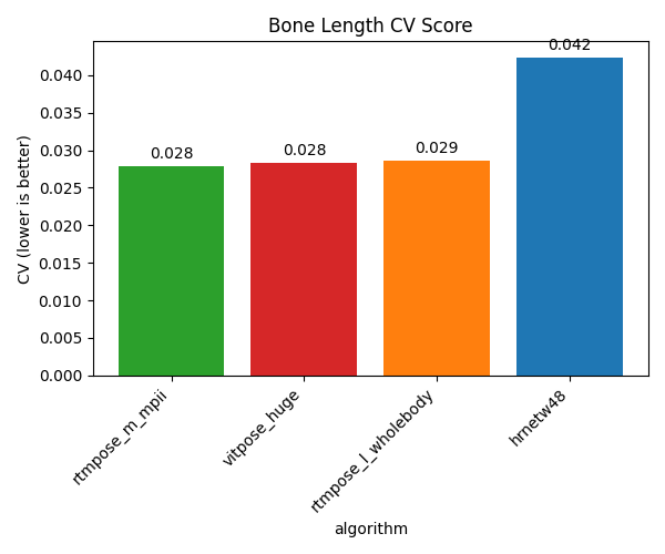
Measures how stable each bone’s length is across all frames for each subject. Real bone lengths are constant, so high variance indicates tracking instability rather than actual movement. Stability is reported as the coefficient of variation (CV = std / mean).
Inputs: 3D keypoint predictions. Bone definitions (which joint pairs form each bone) are read from predictions_mapping.toml.
Key parameters:
predictions: which component and NPZ key to read — must be a 3D keypoint arraysummary_group_by: dimensions to break results down bysummary_aggr: which statistical columns to include in the output CSV
Warning
Always include "subject" in summary_group_by. Bone lengths differ between people, so pooling across subjects produces meaningless variance estimates.
Output — summary CSVs: coefficient_variation_score.csv (one row per algorithm, aggregated across all groups) and summary.csv (full breakdown per summary_group_by dimensions). Columns depend on summary_aggr; common choices are mean, std, cv per bone. Check cv — lower is better.
Output — NPZ arrays: bone_length (per-frame length of each bone), predictions (raw 3D input used).
Aggregation: macro — summary_aggr functions are applied to the per-frame bone length values within each group independently.
[metrics.bone_length]
metric_type = "bone_length"
predictions = { component = "body_joints", npz_key = "3d" }
summary_group_by = ["subject", "sequence", "label"]
summary_aggr = ["mean", "std", "cv"]
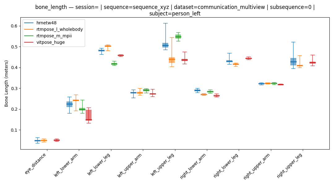
The candle plot shows the distribution of each bone’s length across all frames, grouped by algorithm. Tight boxes indicate stable tracking; wide boxes indicate high variance.
The CV score bar summarises tracking stability per algorithm across all bones — lower is better.
Missing Points
Counts joints that are absent or unreliable per frame. A joint is considered missing if any of its spatial coordinates is NaN, or if its confidence score falls below an optional threshold.
Inputs: 2D or 3D keypoint predictions.
Key parameters:
predictions: component and NPZ key to evaluatemin_confidence(optional): float threshold on the confidence coordinate; joints below this value are treated as missing (e.g.0.5)missing_points_summary_group_by: grouping dimensionsmissing_points_summary_aggr: aggregation functions for the output CSV
Output — summary CSVs: detection_rate_score.csv (one row per algorithm, aggregated across all groups) and summary.csv (full breakdown per missing_points_summary_group_by dimensions). Columns depend on missing_points_summary_aggr; common choice is detection_rate (= 1 − missing rate). Check detection_rate — higher is better.
Output — NPZ arrays: missing (binary flag per joint per frame — 1 if missing, 0 if detected), detected_pct (fraction of joints detected per frame), confidence (raw confidence values), predictions (raw input used).
Aggregation: macro — missing_points_summary_aggr functions are applied to the per-frame missing flags within each group independently.
[metrics.missing_points_3d]
metric_type = "missing_points"
predictions = { component = "body_joints", npz_key = "3d" }
missing_points_summary_group_by = []
missing_points_summary_aggr = [
    { name = "total_count",    fn = "count" },
    { name = "miss_count",     fn = "sum" },
    { name = "detection_rate", fn = "one_minus_mean" }
]
The heatmap shows the detection rate per joint per algorithm. White cells indicate joints not tracked by that algorithm; red indicates frequent misses.

PCK — Percentage of Correct Keypoints
A keypoint is correct if it exists (non-NaN) and its distance to the ground-truth position is within threshold pixels. The metric reports the fraction of correct keypoints.
Inputs: 2D keypoint predictions + ground-truth keypoint annotations.
Key parameters:
threshold: distance threshold in pixels — strict values (e.g.5px) penalise small errors; lenient values (e.g.20px) tolerate more imprecisionpredictions: component and NPZ key for the predictionsground_truth: component and NPZ key for annotations, withsource = "annotation"to indicate this is not a detector output
Output — summary CSVs: pck_score.csv (one row per algorithm, aggregated across all groups) and summary.csv (full breakdown per summary_group_by dimensions). Common columns: pck (fraction of keypoints within the distance threshold), correct_count (number of correct keypoints), support (total number of keypoints evaluated). Check pck — higher is better.
Output — NPZ arrays: pck (per-frame per-joint correctness flag — 1.0 if correct, 0.0 if incorrect or missing), predictions (aligned predictions), ground_truth (aligned GT annotations).
Aggregation: macro — summary_aggr functions (e.g. mean) are applied to the per-frame correctness flags within each group independently.
[metrics."body_pck@5px"]
metric_type = "pck"
threshold = 5
predictions = { component = "body_joints", npz_key = "2d_interpolated" }
ground_truth = { source = "annotation", component = "body_joints", npz_key = "2d" }
summary_group_by = ["label"]
summary_aggr = [
    { name = "pck",           fn = "mean"  },
    { name = "correct_count", fn = "sum"   },
    { name = "support",       fn = "count" }
]
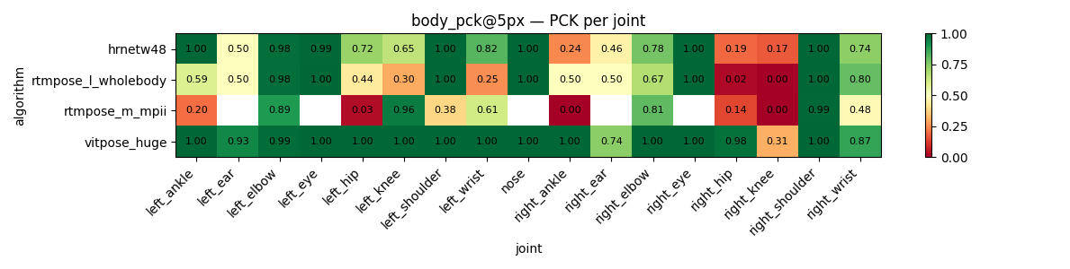
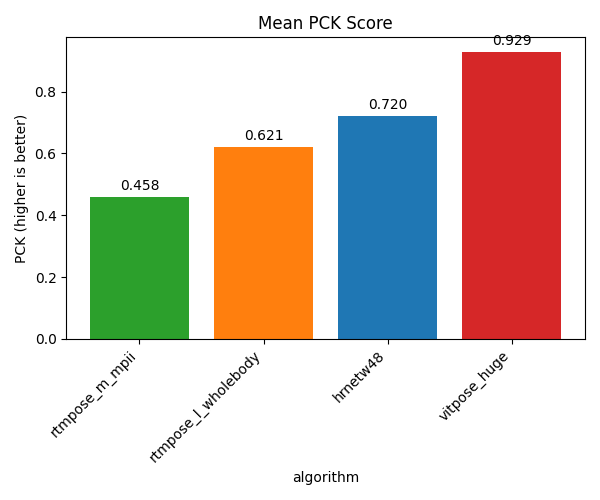
The heatmap shows PCK per joint per algorithm at the configured threshold. The score bar shows the mean PCK across all joints per algorithm.
Distance Error
Computes the direct per-joint distance between predicted and ground-truth positions using either the L2 (Euclidean) or L1 (Manhattan) norm. Unlike PCK, this does not apply a threshold — it gives the raw error value.
Inputs: 2D or 3D keypoint predictions + ground-truth keypoint annotations.
Key parameters:
norm:"l2"(default) or"l1"predictions/ground_truth: component and NPZ key
Output — summary CSVs: mean_error_score.csv (one row per algorithm, aggregated across all groups) and summary.csv (full breakdown per summary_group_by dimensions). Columns depend on summary_aggr; common choices are mean, std, min, max per joint. Check mean — lower is better.
Output — NPZ arrays: distance_error (per-frame per-joint distance to ground truth), predictions (aligned predictions), ground_truth (aligned GT annotations).
Aggregation: macro — summary_aggr functions are applied to the per-frame distance values within each group independently.
Confusion Matrix
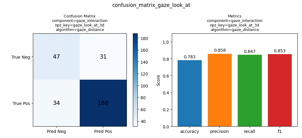
For binary (True/False) prediction arrays, computes a confusion matrix and derives precision, recall, F1, and accuracy. All frames within each group are pooled before computing the matrix — see Micro and Macro Aggregation for details.
Inputs: Boolean prediction array + boolean ground-truth annotation array.
Key parameters:
predictions/ground_truth: component and NPZ key (must contain boolean values)compute_group_by: dimensions used to pool frames before computing the matrix
Output — summary CSV: summary.csv with columns tp, fp, fn, tn, accuracy, precision, recall, f1, support — one row per compute_group_by group.
Output — NPZ arrays: predictions (aligned boolean predictions), ground_truth (aligned boolean GT labels).
Aggregation: micro — all frames within each compute_group_by group are pooled into a single pool first, then the confusion matrix is computed once on that pool. A larger group has proportionally more weight than a smaller one.
[metrics.confusion_matrix_gaze]
metric_type = "confusion_matrix"
predictions = { component = "gaze_interaction", npz_key = "gaze_look_at_3d" }
ground_truth = { source = "annotation", component = "gaze_interaction", npz_key = "gaze_look_at_3d" }
compute_group_by = []
The visualisation shows the confusion matrix alongside derived accuracy, precision, recall, and F1 scores.
ROC AUC
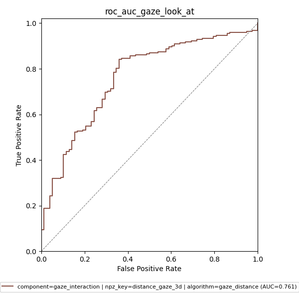
Computes the Receiver Operating Characteristic (ROC) curve and the Area Under the Curve (AUC) by sweeping all possible decision thresholds. AUC measures how well the model ranks positives above negatives regardless of the chosen threshold. Also reports the optimal threshold via Youden’s J statistic (maximises TPR − FPR). Suitable when predictions are continuous scores rather than hard boolean decisions.
Inputs: Float confidence scores (predictions) + boolean ground-truth labels.
Key parameters:
predictions/ground_truth: component and NPZ keynegate_scores: settruewhen a lower score indicates a positive — for example, a gaze distance metric where a smaller distance means “looking at”compute_group_by: dimensions used to pool frames before computing the curve
Output — summary CSV: summary.csv with columns auc, optimal_threshold, support — one row per compute_group_by group. Check auc — higher is better (1.0 = perfect, 0.5 = random).
Output — NPZ arrays: predictions (aligned float scores), ground_truth (aligned boolean GT labels).
Aggregation: micro — all frames within each compute_group_by group are pooled first, then the ROC curve and AUC are computed once on that pool.
[metrics.roc_auc_gaze]
metric_type = "roc_auc"
predictions = { component = "gaze_interaction", npz_key = "distance_gaze_3d" }
ground_truth = { source = "annotation", component = "gaze_interaction", npz_key = "gaze_look_at_3d" }
negate_scores = true  # larger distance = not looking
compute_group_by = []
PR Curve — Average Precision
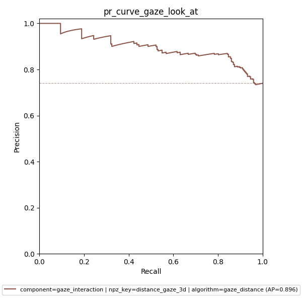
Computes the Precision-Recall curve and the Average Precision (AP) score by sweeping decision thresholds. AP is often preferred over ROC AUC when positive and negative classes are heavily imbalanced, because it focuses on the positive class. Also reports the decision threshold that maximises F1 across the curve.
Inputs: Float confidence scores (predictions) + boolean ground-truth labels.
Key parameters:
predictions/ground_truth: component and NPZ keynegate_scores: same meaning as in ROC AUCcompute_group_by: dimensions used to pool frames
Output — summary CSV: summary.csv with columns ap, optimal_threshold, support, prevalence — one row per compute_group_by group. Check ap — higher is better.
Output — NPZ arrays: predictions (aligned float scores), ground_truth (aligned boolean GT labels).
Aggregation: micro — all frames within each compute_group_by group are pooled first, then the PR curve and AP are computed once on that pool.
[metrics.pr_curve_gaze]
metric_type = "pr_curve"
predictions = { component = "gaze_interaction", npz_key = "distance_gaze_3d" }
ground_truth = { source = "annotation", component = "gaze_interaction", npz_key = "gaze_look_at_3d" }
negate_scores = true
compute_group_by = []
Aggregation
Aggregation Functions
The summary_aggr parameter selects which statistical columns appear in the output CSV. You can either list function names directly (the column name will match the function) or provide custom column names via { name = "...", fn = "..." }.
Function |
Description |
|---|---|
|
Average value |
|
Standard deviation |
|
Minimum / maximum |
|
Total — useful for counting correct frames |
|
Number of samples (total frames evaluated) |
|
50th percentile |
|
25th / 75th / 90th percentile |
|
Coefficient of variation (std / mean) |
|
1 − mean — use to report detection rate instead of missing rate |
# shorthand: column name matches function name
summary_aggr = ["mean", "std", "cv"]

# custom column names
summary_aggr = [
    { name = "detection_rate", fn = "one_minus_mean" },
    { name = "support",        fn = "count" }
]